Ir al contenido
Ecuación de Taylor para la vida útil de la herramienta: calcula n y C, y luego comprueba el resultado
The Taylor equation for tool life, VT^n = C, estimates how long a tool will cut at a given cutting speed. To use it, you need speed-life data from the same tool, work material, setup, cutting conditions, and end-of-life criterion. The worked example below shows how to calculate n y C; the trial guidance explains how to decide whether your own fitted equation is reliable.
The practical sequence is simple: define what failure means, hold the other variables steady, vary cutting speed, measure life to the same criterion, fit the local relationship, and check its prediction at a speed not used in the fit. Only then should the result enter a production decision about cycle time, tool changes, quality, and cost per part.
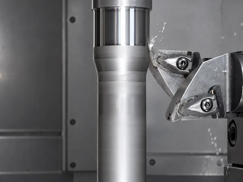
What the Taylor tool life equation means
In the basic relationship, V es la velocidad de corte, T is tool life, n is the slope-related exponent, and C is a fitted constant. The variables need declared units and a declared process. The equation says that, for the tested domain, a change in speed is associated with a change in life. It does not identify the wear mechanism by itself, and it does not replace a tool-life definition.
The log form makes the fitting step visible:
log V = log C - n log T
A straight-line relationship in log-log space is therefore a useful first model. A fitted line is not proof that every point belongs to one regime. A change in built-up edge behavior, thermal condition, interruption, workholding, or tool state can make the slope change. The model is a description of the trial, not permission to extrapolate indefinitely. This condition-bounded interpretation follows the machining teaching material and reviewed evidence from NPTEL, IIT Bombay, and a tool-life study.
Define tool life before cutting
Tool life is the elapsed cutting time, or another declared production measure, until a specified end condition. The end-of-life criterion is part of the experiment. If one point ends at a visible flank-wear limit and another ends after a finish or tolerance failure, their life values do not describe the same dependent variable.
Pick one end-of-life criterion
Choose a criterion that the shop can observe consistently and that matters to the operation. Depending on the process, it may be a measured wear limit, crater wear, loss of surface finish, loss of dimensional tolerance, a force or vibration threshold, or a controlled breakage condition. Research work may monitor more than one signal, but the fitted life value still needs one declared rule.
Write the rule before the first cut. Include the measurement method, the sampling interval, and what happens if a tool fails catastrophically before reaching the planned observation. The same rule must be applied at each speed. Otherwise, the fitted slope may describe a change in inspection practice rather than a change in cutting speed.
Record conditions that make life comparable
The trial record should make it possible for another engineer to tell whether two points belong to the same experiment. The following fields are more valuable than a single life number:
| Field group | Why it matters to the trial |
|---|---|
| Work material, condition, and batch | A material name alone may not identify the cutting response. |
| Tool grade, diameter or insert identity, edge preparation, geometry, and coating | Life belongs to the actual tool-work pair, not to a generic label. |
| Machine, spindle, workholding, rigidity, runout, and stickout | Setup behavior can change load, vibration, and heat. |
| Feed, axial and radial engagement, depth of cut, toolpath or cut type, and coolant | These are held factors in a speed-only trial and must be repeatable. |
| Cutting speed, measured life, end-of-life result, and observation method | This is the minimum traceable speed-life record. |

Build the controlled cutting-speed trial
Use a speed-only design first when the question is whether the basic Taylor relationship is useful for the operation.
- Choose what to measure. Decide whether the response is minutes in cut, parts per edge, cut length, or another production measure. Set the end-of-life criterion and the quality checks before cutting.
- Record the test conditions. Record the work material and condition, tool identity and geometry, machine and setup, feed, engagement, depth, coolant, measurement method, and any interruption or toolpath pattern.
- Select bounded speed levels. Choose levels that test the operating window you care about. Do not choose an extreme point merely to create a dramatic slope, and do not assume the fitted line is valid outside the tested range.
- Change speed first. Keep the other declared factors fixed. If feed, depth, coolant, edge preparation, or toolpath changes with speed, label the work as a different experiment rather than combining the points.
- Measure to the same rule. Record life and the actual reason the tool stopped. Note breakage, finish, tolerance, vibration, chip behavior, and other anomalies as observations, not as replacements for the defined criterion.
- Repeat where the decision justifies it. Replication helps separate ordinary scatter from a speed effect. It is especially important when a tool change, scrap event, or customer-facing quality risk is expensive.
Two speed-life points can solve for a line algebraically, but that is an educational minimum, not industrial validation. More points help reveal scatter, curvature, and a failed assumption.
A controlled tool-life trial
- Define the endpoint. Use one observable end-of-life rule.
- Fix the conditions. Identify the tool, material, setup, feed, engagement and coolant.
- Vary cutting speed. Select bounded levels for the same experiment.
- Measure life. Keep raw observations, repeats and anomalies.
- Fit n and C. Inspect scatter and possible regime changes.
- Validate separately. Compare a new in-range cut with the prediction.
- Evaluate production. Include quality, cycle time and cost per part.
Fit the equation and test its limits
For each valid point, transform the measured speed and life into log values and fit log V against log T. In this arrangement, the fitted slope is -n and the intercept is log C. Keep the raw values beside the transformed values. You will need those values to check unusual points or repeat the calculation.
Check more than the coefficient of determination. Inspect residuals, repeated points, the distribution of failures, and whether the line bends at one part of the speed range. Ask whether the same wear mode, measurement method, and process engagement applied throughout. If a point ends by a different mechanism, mark it and investigate before forcing it into the fit.
Worked example: calculate n, C, and a predicted tool life
Purdue’s machining teaching example supplies two speed-life points for turning, with feed fixed at 0.025 in/rev, depth of cut at 0.015 in, workpiece diameter 2 in, and cut length 10 in:
| Cutting speed V (ft/min) | Tool life T (min) |
|---|---|
| 350 | 60 |
| 500 | 10 |
These are teaching-problem inputs, not recommended settings or SCT test results. The problem does not identify the tool grade, work material, or wear limit needed to transfer the result to a shop operation.
1. Solve for n. Both points share the same C, so:
350 × 60^n = 500 × 10^n
n = ln(500/350) / ln(60/10) ≈ 0.199064
2. Solve for C. Substitute either point, retaining the unrounded value of n:
C = 350 × 60^n ≈ 790.741
Utilice V in ft/min and T in minutes with this constant. Changing the speed unit changes the numerical value of C. The source solution rounds n to 0.2 before calculating C; the values here retain precision until the final display.
3. Predict life at an intermediate speed. Choose 425 ft/min solely to illustrate a prediction inside the two-point range:
T = (C/V)^(1/n) = (790.740678…/425)^(1/0.199064076…) ≈ 22.62 min
That is a calculated estimate, not an observed result. For a real trial, a separate cut at that speed would have to reach the same end-of-life criterion under the same conditions. Compare its measured life and quality with the prediction, and repeat as needed to assess scatter. A two-point line passes through both input points by construction; that alone cannot validate it.
Taylor tool life calculator
Enter two comparable speed–life measurements to calculate n and C, then estimate life at another speed. Use cutting time in minutes and one speed unit throughout.
- Exponent n
- —
- Constant C
- —
- Predicted tool life
- —
Enter two speed–life points.
n = ln(V₂/V₁) / ln(T₁/T₂); C = V₁T₁ⁿ; T = (C/V)¹/ⁿ. C uses the selected speed unit and minutes raised to n. Two points fit a line exactly; they do not validate the model. Keep tool, work material, setup and end-of-life criterion comparable, and check a separate measured point before production use. Example values are teaching inputs, not cutting recommendations.
Look for regime changes and failed assumptions
A single Taylor line becomes questionable when the operating regime changes. Warning signs include built-up edge appearing or disappearing, a thermal or lubrication shift, intermittent cutting, chatter, sudden fracture, a new chip form, or a monitoring signal that no longer follows the earlier pattern. These signs do not automatically tell you which model is correct. They tell you to stop treating the points as one homogeneous set.
Use the fitted relationship only inside the region where the observations support it. Validate with a speed that was not used to calculate the line, then compare predicted and observed life under the same end-of-life rule. If validation fails, narrow the domain, split the regimes, add controlled data, or stop using the model for that decision.
Extend the model only when the design supports it
If feed and depth must be studied as well, a modified form can be written as V_c T^n f^m d^k = C, with the variables and units declared. This is an empirical extension. It requires a design that changes and estimates those factors, not a base speed trial with extra symbols added afterward.
Fit the additional exponents from measurements that vary feed and depth as part of a planned experiment. Keep the tool, work material, machine, coolant, operation and wear criterion with the fitted values. Coefficients from a different experiment cannot substitute for that validation. The dimensions and numerical value of C depend on the variables and units, so a copied constant without its model and unit system is not usable cutting guidance.
Turn tool life into a production decision
The longest observed life is not automatically the lowest-cost choice. A higher speed may reduce cycle time but increase tool changes, inspection, scrap exposure, or instability. A slower speed may consume more machine time but reduce interruptions. The decision should compare the whole part-making result under the conditions actually validated.
At minimum, place these measures beside the fitted life estimate:
- cycle time and productive cutting time;
- tool cost and tool-change time;
- parts or cut length per edge;
- dimensional and surface-finish results;
- scrap, rework, and interruption risk;
- setup and operator burden for the intended production quantity.
Use the validated tool-life estimate in an economic decision that also accounts for print requirements, machine condition, tool-change timing and measured production results. A starting chart and an in-house trial have different evidential value. Tool life is a production variable whose usefulness depends on the quality and cost outcome of the complete operation.
Before using the result in production
Before changing a production plan, confirm that:
- the tool, work material, machine, setup, engagement, coolant, and measurement method are identified;
- every fitted point uses the same end-of-life criterion;
- raw observations, anomalies, and repeated points are retained;
- the fitted range and any regime changes are documented;
- an in-range validation point has been observed;
- cost per part and quality results support the proposed choice.
If any item is missing, the result may still be useful for planning the next trial, but it is not yet a production setting.
Conclusión
Calcular n y C from comparable speed-life data, then check a prediction against a separate cut within the fitted range. If the prediction and the quality results hold up, use the estimate alongside cycle time, tool-change time, and cost per part. The useful result is not a universal constant; it is a tested choice for your operation.